Addendum after hitting the HN frontpage: MNIST is a straightforward dataset, and higher accuracies are possible with various methods. The novelty of this post isn't aiming for state-of-the-art results, but showcasing the potential of using compression as a unique, model-free classification tool. The code golf just adds a layer of complexity for fun.

We can 'solve' MNIST up to ~78% accuracy with the following code-golfed obscurity:

c = lambda z: len(gzip.compress(z.tobytes()))

def ncd(x, y):
    return (c(x + y) - min(c(x), c(y))) / max(c(x), c(y))

cls = [(x, c(x), l) for x, l in training_set]

correct_predictions = sum([np.array_equal(Counter(
    [l for _, _, l in sorted([(ncd(x1, x), x, l) for x, _, l in cls],
     key=lambda t: t[0])[:5]]).most_common(1)[0][0], label)
     for x1, label in test_set])

If you just want to see the code sample, here is a link to the Jupyter Notebook containing the code to run this experiment.

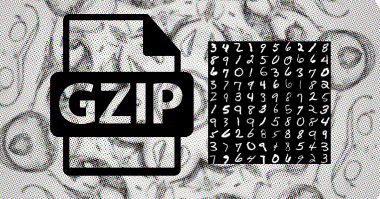
Lets dive into why and how: yesterday while in the one-hour train ride from Eindhoven to Rotterdam, I was inspired by the post text generation from data compression and the (quite controversial) paper on parameter free text classification to play around with using compression as an image classification mechanism. Previously, I worked on image compression for computer vision on the edge, so interested in applying the technique to the most seminal yet basic dataset, I attempted to use GZIP + K-NN as a classification mechanism for the MNIST (handwritten digits) dataset.

Breaking down the technique, it boils down to two components: GZIP and NCD (Normalized Compression Distance) as a similarity metric, and k-NN (k-Nearest Neighbors) for classification. In this approach, GZIP is essentially our tool which gives us a way to measure the complexity or information content of individual data points. NCD provides a normalized measure of how similar two data points are, based on how much more (or less) effort it takes to compress them together compared to compressing them separately.

For each test sample, the algorithm computes its NCD with every training sample (in our case, 100 training samples), sorts them, and selects the k smallest distances. The majority class among these k=5 closest neighbors is then predicted as the label for the test sample. As this is quite computationally expensive, I only took a subset of the test images to arrive at my accuracy measure. Of course, it would be more correct to use the full set, but I leave this an an exercise to the reader ;).

Here is a less obscured version of the algorithm:

def compute_ncd(x1, x2):
    """Compute the Normalized Compression Distance (NCD) between two samples."""
    Cx1 = len(gzip.compress(x1.tobytes()))
    Cx2 = len(gzip.compress(x2.tobytes()))
    Cx1x2 = len(gzip.compress((x1 + x2).tobytes()))
    
    return (Cx1x2 - min(Cx1, Cx2)) / max(Cx1, Cx2)

print("Classifying test samples...")

k = 5  # Number of neighbors to consider
correct_predictions = 0  # Counter for correct predictions
actual_labels = []
predicted_labels = []

# Cache compressed lengths for training samples
compressed_lengths = [(x, len(gzip.compress(x.tobytes())), label) for x, label in training_set]

for (x1, actual_label) in tqdm(test_set[:100]):
    # Calculate NCD for each training sample
    distances = [(compute_ncd(x1, x), label) for x, _, label in compressed_lengths]
    
    # Get k nearest neighbors and predict label
    neighbors = sorted(distances, key=lambda x: x[0])[:k]
    top_k_class = [label for _, label in neighbors]
    predicted_class = Counter(top_k_class).most_common(1)[0][0]
    
    # Update predictions and counts
    actual_labels.append(actual_label)
    predicted_labels.append(predicted_class)
    correct_predictions += (predicted_class == actual_label)

Note: after writing this post, I found this article by Andreas Kirsch taking a similar approach back in 2019.

Note 2: Recently emailed by a reader: I ignore the cached compressed values completely. Looking back, I probably missed this when refactoring my notebook into a 'clean' example. Thanks for pointing it out! reader's message:

you've probably had this pointed out already, but I just realized one thing: both in the "regular" and "obfuscated" versions, you compute a cache of compressed lengths for every entry in your training set, but then proceed to ignore the cached values completely (e.g. for x, _, label in compressed_lengths / for x, _, l in cls). It kinda bugged me so I just wanted to point it out, i.e. it would satisfy my OCD if you got rid of the cache and just straight up use x, l in training_set in the main prediction loop, or somehow feed it into compute_ncd to utilize it :)